Datasets

Biometrics Dataset: contains nine skeletal measurements and twelve girth measurements along with age, weight, height, and gender.

Cancer Dataset: contains data on tumor types and hypermethylation genes

Compliance Dataset: dataset of treatment compliance for a 10-week study on physical activity and cognitive functioning.

OCD Dataset: dataset of a small observational study on OCD. Patients were measured using the YBOCS scale over eight months.

NYC COVID-19 Dataset: US State-level COVID-19 dataset from the New York Times data portal.

# Biometrics dataset
biometrics_raw <- read_excel('Datasets/biometrics.xls', sheet = 2)

# Cancer dataset
cancer <- read_csv('Datasets/cancer_genes.csv', skip = 2) %>%
  drop_na(hyper_methylation) 

# Compliance dataset
compliance <- read_csv('Datasets/activity_compliance.csv') %>%
  mutate(compliant = if_else(is.na(compliant), 0, compliant))

# OCD dataset
ocd_longitudinal <- read_csv('Datasets/ocd_longitudinal.csv')
ocd_demos <- read_csv('Datasets/ocd_demos.csv')

# COVID-19 dataset
covid_raw <- read_csv("https://raw.githubusercontent.com/nytimes/covid-19-data/master/us-states.csv")

Data Manipulation

Filter and create new variables

# biometrics dataset manipulation
biometrics_girth <- biometrics_raw %>%
# filter to selected variables - demography and all girth measurements
  select(id, height, weight, gender, contains("girth")) %>%
  
# create new calculated variables
  mutate(bmi = round(weight/(height/100)^2,1)) %>%  #BMI
  mutate(navel_thigh_girth = navel_girth + thigh_girth) %>% # combined navel, thigh girth

# create categorical variable for BMI
  mutate(bmi_cat = case_when(bmi < 18.5 ~ "Underweight",
                             bmi >=18.5 & bmi < 25 ~ "Normal",
                             bmi >=25 & bmi < 30 ~ "Overweight",
                             bmi >= 30 ~ "Obese")) %>%

# factor categorical variables
  mutate(bmi_fac = factor(bmi_cat, levels = c("Underweight","Normal", "Overweight",
                                              "Obese")))

Summarize data

# compliance dataset summarization of proportion by week:
proportion_by_week <- compliance %>% 
  group_by(week, compliant) %>%
  summarize(n = n()) %>%
  mutate(compliance_proportion = n / sum(n),
         sd = sd(compliance_proportion),
         se = sd/(sqrt(n)),
         lower_ci = compliance_proportion - (1.96*se),
         upper_ci = compliance_proportion + (1.96*se)) %>%
  filter(compliant == 1) %>%
  select(week, compliance_proportion, lower_ci, upper_ci)

# print results
kable(proportion_by_week)

week	compliance_proportion	lower_ci	upper_ci
1	0.8000000	0.6799750	0.9200250
2	0.7500000	0.6466989	0.8533011
3	0.6500000	0.5834221	0.7165779
4	0.7500000	0.6466989	0.8533011
5	0.5666667	0.5349753	0.5983580
6	0.5166667	0.5083693	0.5249640
7	0.4666667	0.4492056	0.4841277
8	0.6666667	0.5936218	0.7397116
9	0.6166667	0.5635027	0.6698306
10	0.5166667	0.5083693	0.5249640

Joins

# inner join OCD dataset
ocd <- inner_join(ocd_longitudinal, ocd_demos, by = "study_id")

Pivot data and String manipulation

# pivot ocd dataset longer
ocd_long <- ocd %>%
  pivot_longer(cols = starts_with("ybocs"),
               names_to = "month",
               values_to = "ybocs_score",
               names_transform = list("month" = function(str){
                 step1 <- str_remove(str, "ybocs_m")  # remove prefix
                 step2 <- as.numeric(step1)   # code month as numeric
                 return(step2)
               })) %>%
# create remission variable
  mutate(remission = if_else(ybocs_score <= 15, "1", "0")) %>%
  # factor remission variable and study_id for visualization
  arrange(study_id) %>%
  mutate(study_id = factor(study_id, levels = unique(study_id)),
         rem_fac = factor(remission, levels = c(0, 1))) %>%
# create age categorical variable
  mutate(age_cat = if_else(age < 18, "minor", "adult"))

Statistical Analysis

T test

# example t-test between ankle diameter measure and gender

# unequal variance
ankle_res <- t.test(ankle_diameter ~ gender, data = biometrics_raw)

# pull results to objects
t_stat <- ankle_res$statistic   # t statistic
df <- ankle_res$parameter   # degrees of freedom
p_val <- ankle_res$p.value  # p-value
ci_lower <- ankle_res$conf.int[1]  # 95% confidence interval
ci_upper <- ankle_res$conf.int[2]

# create tibble of results and print
ankle_res_tidy <- tidy(ankle_res)
kable(ankle_res_tidy)

estimate	estimate1	estimate2	statistic	p.value	parameter	conf.low	conf.high	method	alternative
-1.717591	13.02654	14.74413	-21.3131	0	495.6447	-1.875928	-1.559254	Welch Two Sample t-test	two.sided

# interpret using in-line code

Interpretation: At the 5% level of significance, we reject the null hypothesis that there is no mean difference in ankle diameter between gender groups (t=-21.31, df=495.64, p<0.0001). We are 95% confident that the true mean difference in ankle diameter between females and males lies between -1.88 and -1.56.

Permutation Test (and function writing)

# create a function to calculate the test statistic
calculate_ts <- function(df){
  summary <- df %>%
    group_by(gender) %>%
    summarize(mean_ank = mean(ankle_diameter))

  female_ank <- summary %>%
    filter(gender == "Female") %>%
    pull(mean_ank)

  male_ank <- summary %>%
    filter(gender == "Male") %>%
    pull(mean_ank)

  difference <- female_ank - male_ank
  return(difference)
}

# calculate observed test statistic with function
obs_stat <- calculate_ts(biometrics_raw)

# create a function to perform a single permutation
perform_permutation <- function(df){
  permuted <- df %>%
    mutate(gender = sample(gender)) # performs a permutation with sample()
  return(permuted)
}

# combine functions
get_permutation_ts <- function(df){
  permed <- perform_permutation(df)
  ts <- calculate_ts(permed)
  return(ts)
}

# simulate 2000 test statistics with map function
results <- map_dbl(1:2000, function(x) get_permutation_ts(biometrics_raw))
# put results into a tibble
perm_results <- tibble(sim_stat = results)

# calculate p-value - proportion of simulated test statistics whose absolute value is greater than or equal to the observed test statistic
perm_pval <- perm_results %>%
  mutate(abs_val_greater = if_else(abs(sim_stat) >= abs(obs_stat), 1, 0)) %>%
  group_by(abs_val_greater) %>%
  summarize(n_obs = n()) %>%
  mutate(proportion = n_obs/sum(n_obs)) %>%
  filter(abs_val_greater == 1) %>%
  pull(proportion)


# create histogram comparing permuted test statistics to the observed difference in means
ggplot(data = perm_results) +
  geom_histogram(aes(x = sim_stat), fill = "darkgrey", color = "white") +
  geom_vline(aes(xintercept = obs_stat), color = "red", linetype = "dashed") +
  theme_bw() +
  labs(x = "Simulated Test Statistics", y = "Count") +
  annotate(geom = "text", x = -0.8, y = 410, label = "Observed Test Statistic = -1.72", color = "red")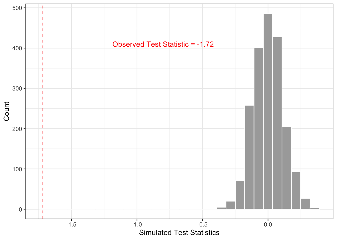

Interpretation: At the 5% level of significance, we reject the null hypothesis that there is no mean difference in ankle diameter between gender groups (p<0.0001).

Regression

# create binary outcomes overweight and obese for logistic regression
biometrics_log <- biometrics_raw %>%
  mutate(bmi = round(weight/(height/100)^2,1)) %>%
  mutate(overweight = if_else(bmi >=25, 1, 0),
         obese = if_else(bmi >=30, 1, 0))

### COVARIATE EXPLORATION ###
# overweight outcome, thigh girth predictor, adjusted for gender
thigh_overweight <- glm(overweight ~ thigh_girth + gender, family = "binomial", 
                        data = biometrics_log)

# obese outcome, thigh girth predictor, adjusted for gender
thigh_obese <- glm(obese ~ thigh_girth + gender, family = "binomial", 
                        data = biometrics_log)

# overweight outcome, wrist girth predictor, adjusted for gender
wrist_overweight <- glm(overweight ~ wrist_girth + gender, family = "binomial", 
                        data = biometrics_log)

# obese outcome, wrist girth predictor, adjusted for gender
wrist_obese <- glm(obese ~ wrist_girth + gender, family = "binomial", 
                        data = biometrics_log)

# overweight outcome, waist girth predictor, adjusted for gender
waist_overweight <- glm(overweight ~ waist_girth + gender, family = "binomial", 
                        data = biometrics_log)

# obese outcome, waist girth predictor, adjusted for gender
waist_obese <- glm(obese ~ waist_girth + gender, family = "binomial", 
                        data = biometrics_log)
tbl_regression(waist_obese, exponentiate = TRUE)

Characteristic	OR¹	95% CI¹	p-value
waist_girth	1.30	1.21, 1.43	<0.001
gender
Female	—	—
Male	0.02	0.00, 0.11	<0.001
¹ OR = Odds Ratio, CI = Confidence Interval

# exploratory results visualized in FOREST PLOT

Example Interpretation: At the 5% level of significance, we reject the null hypothesis that there is no significant difference in waist girth between those who are obese (BMI>=30) and those who are not obese (p=<0.001). For every 1cm increase in waist girth, the odds of being obese increases by a factor of 1.30 on average, adjusting for gender.

### MULTIVARIATE LOGISTIC MODEL ###

mult_obese <- glm(obese ~ waist_girth + wrist_girth + thigh_girth + gender, 
                  family = "binomial", data = biometrics_log)

tbl_regression(mult_obese, exponentiate = TRUE)

Characteristic	OR¹	95% CI¹	p-value
waist_girth	1.31	1.19, 1.49	<0.001
wrist_girth	0.94	0.43, 2.04	0.9
thigh_girth	1.32	1.15, 1.56	<0.001
gender
Female	—	—
Male	0.04	0.00, 0.37	0.006
¹ OR = Odds Ratio, CI = Confidence Interval

Visualizations

Histograms

# graph of distribution of combined navel and thigh girth variable
ggplot(data = biometrics_girth) +
  geom_histogram(aes(x = navel_thigh_girth), color = "white", fill='darkgrey') +
  theme_bw() +
  labs(title = "Distribution of Combined Navel and Thigh Girth", x = "Navel and Thigh Girth", y = "Count")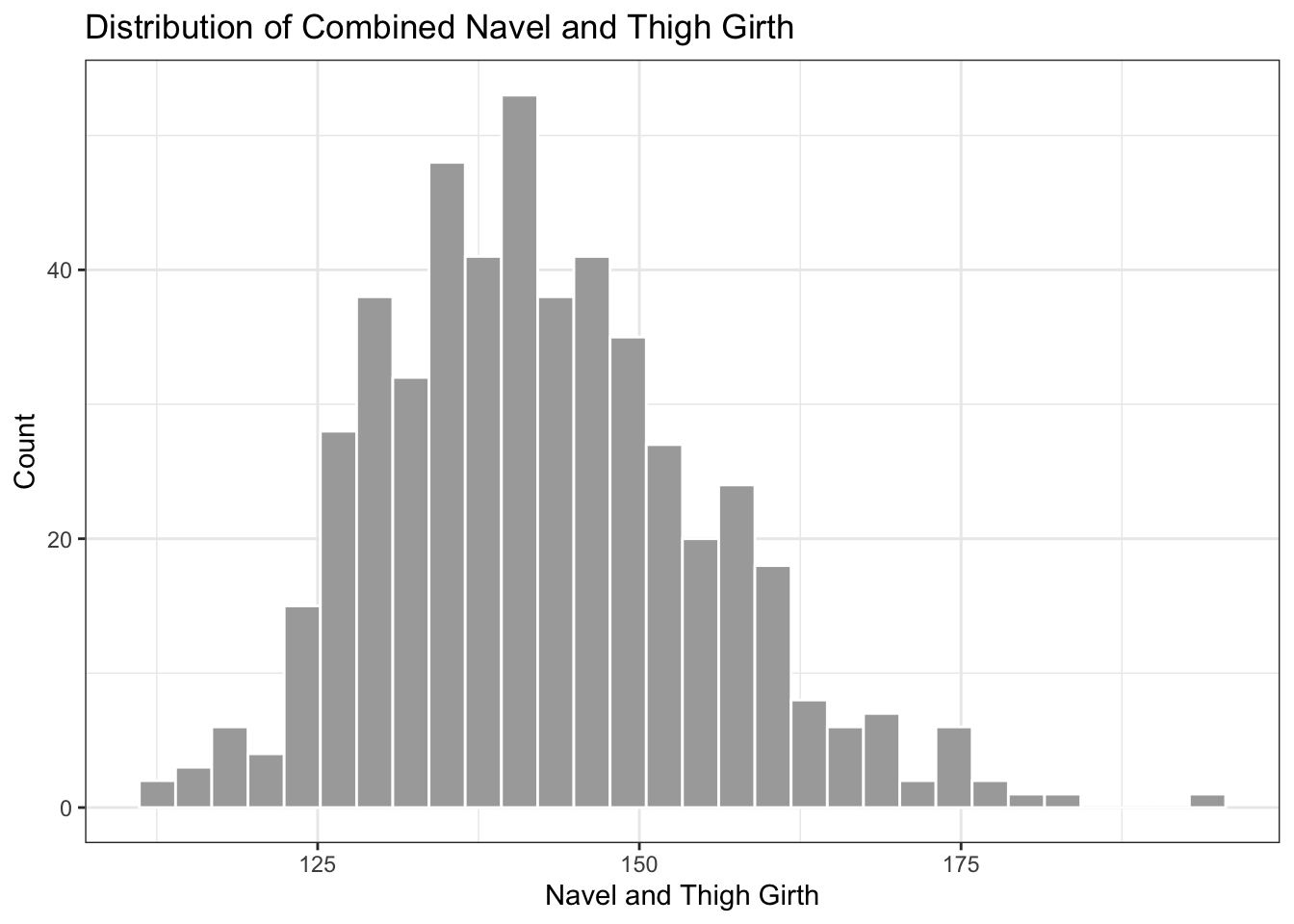

Boxplots

# distribution of combined navel and thigh girth variable, divided by gender
ggplot(data = biometrics_girth) +
  geom_boxplot(aes(y = navel_thigh_girth, x = gender), fill='darkgrey') +
  theme_bw() +
  labs(title = "Distribution of Combined Navel and Thigh Girth", 
       y = "Navel and Thigh Girth", x = "Gender")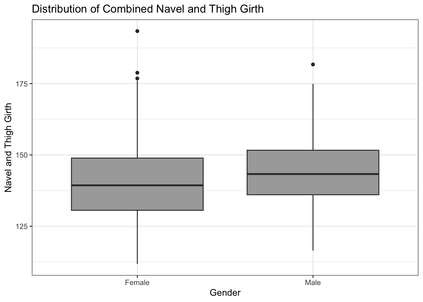

Scatterplots

# exploratory scatterplot for the relationship between continuous BMI and navel+thigh combined girth variable
ggplot(data = biometrics_girth) +
  # scatterplot
  geom_point(aes(x = bmi, y = navel_thigh_girth)) + 
  # linear best fit line
  geom_smooth(aes(x = bmi, y = navel_thigh_girth), method = 'lm', se = FALSE, 
              color = 'red') +
  labs(title = "Relationship between BMI and Combined Navel and Thigh Girth", 
       y = "Navel and Thigh Girth", x = "BMI") + 
  theme_bw()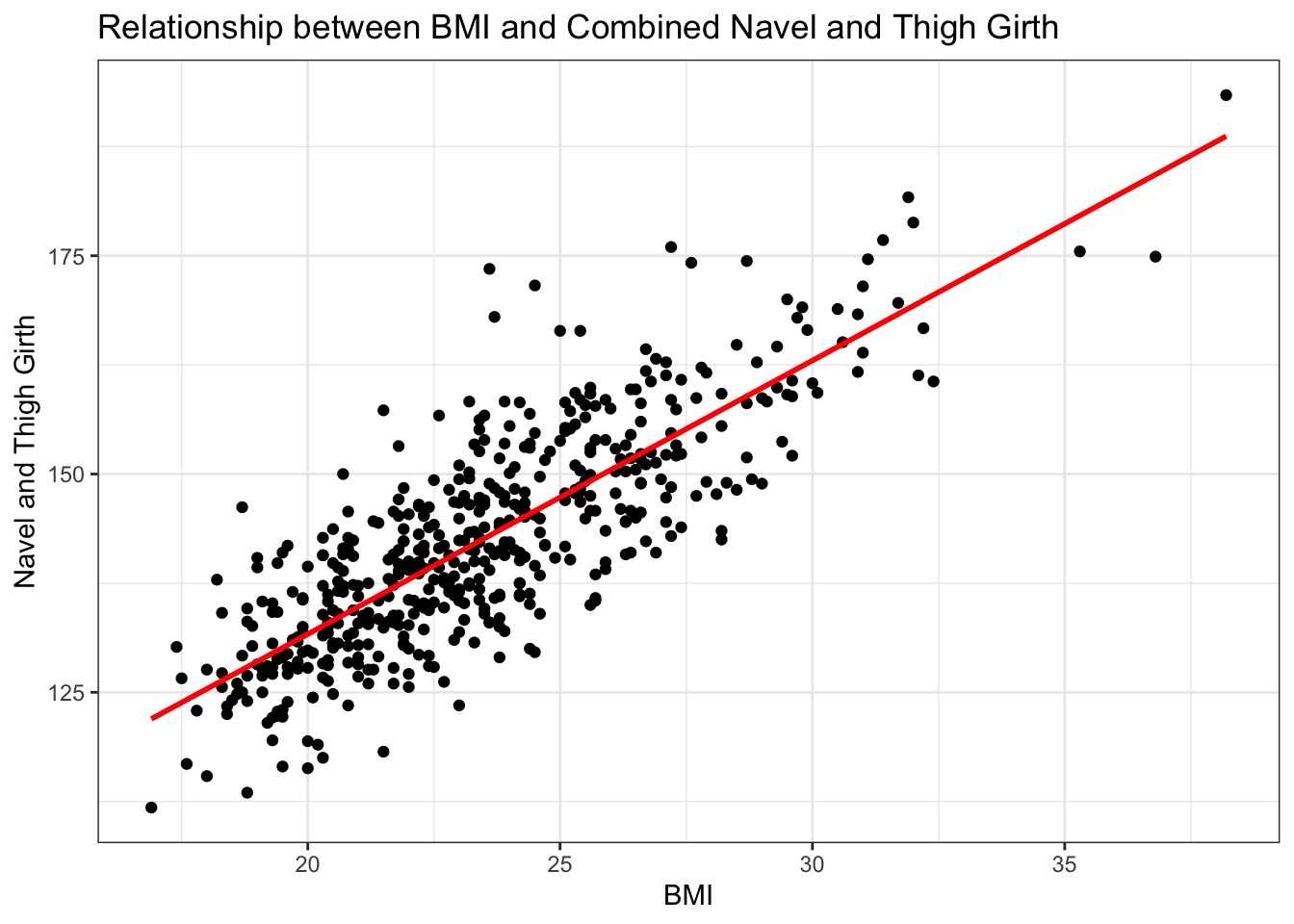

# faceted scatterplots of BMI and navel+thigh combined girth by BMI category and gender
ggplot(data = biometrics_girth) +
  geom_point(aes(x = bmi, y = navel_thigh_girth)) + 
  geom_smooth(aes(x = bmi, y = navel_thigh_girth), method = 'lm', se = FALSE, 
              color = 'red') +
  facet_grid(bmi_fac~gender) + 
  theme_bw() +
  labs(title = "Relationship between BMI and Combined Navel and Thigh Girth,", subtitle= "by BMI category and gender", y = "Combined Navel and Thigh Girth", x = "BMI")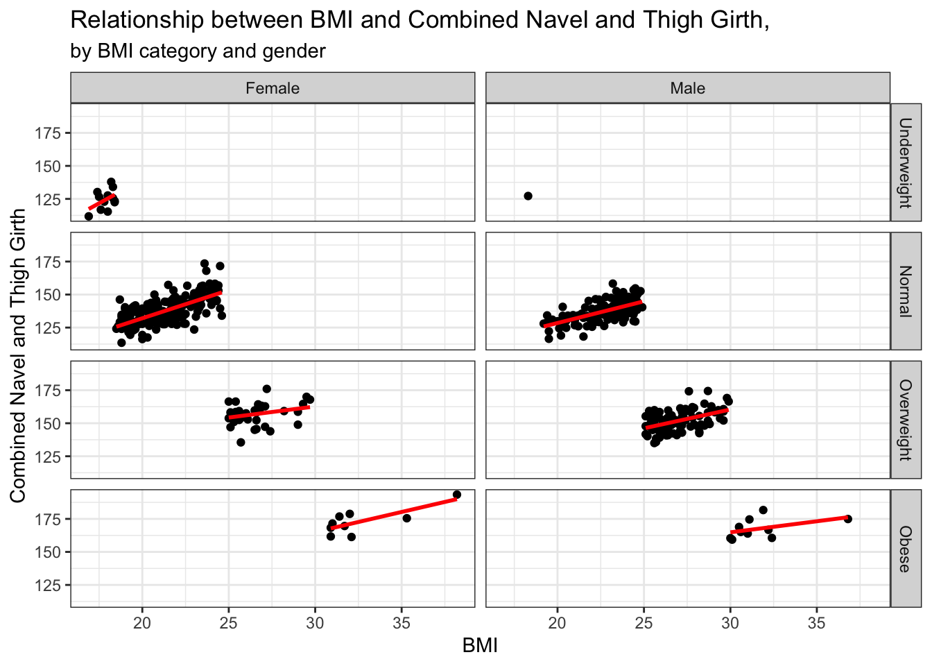

Heatmaps

# heatmap of tumor types and genes, with color indicating severity of hypermethylation in cancer dataset
ggplot(data = cancer) +
  geom_tile(aes(y = tumor_type, x = gene, fill = hyper_methylation)) +
  labs(y = "Tumor Type", x = "Gene", fill = "Hyper Methylation", title = "Hyper Methylation Values by Tumor Type and Gene") +
  theme(axis.text.x = element_text(angle = 90)) + 
  scale_fill_gradient(high = "darkred", low = "white")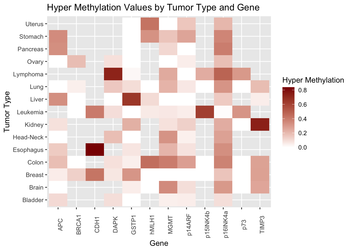

Spaghetti Plots

# spaghetti plot showing YBOCS scores over time for all individuals in OCD dataset
ggplot(data = ocd_long) +
  geom_line(aes(x = month, y = ybocs_score, group = study_id), alpha=0.5) + 
  theme_bw() +
  labs(x = "Month", y = "YBOCS Score", title = "Patient YBOCS Scores by Month") +
  scale_x_continuous(breaks = 1:8, labels = scales::label_number(prefix = "Month "))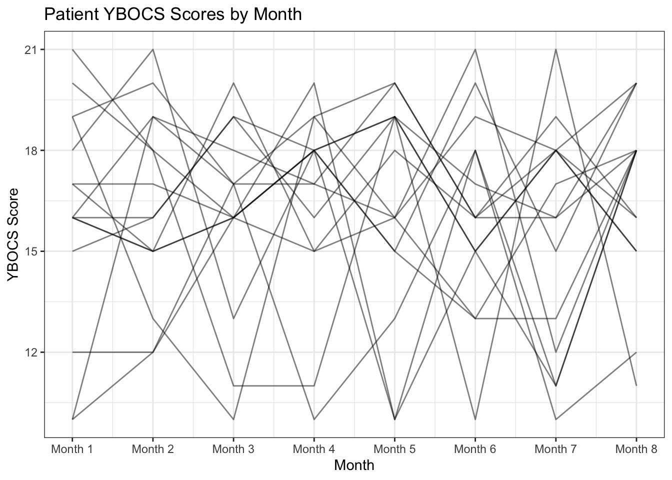

Lasagna Plots

# plot showing the binary remission variable over time for each individual, factored by minor status
ggplot(data = ocd_long) +
  geom_tile(aes(x = month, y = study_id, fill = rem_fac), color = "black") +
  labs(x = "Month", y = "Patient ID", title = "Patient Remission Status by Month",
       fill = "Remission Status") +
  theme(legend.position = "bottom",
        panel.background = element_rect(fill="white")) +
  scale_x_continuous(breaks = 1:8) +
  scale_fill_manual(values = c("grey", "darkblue")) +
  facet_wrap(~age_cat, scales = "free")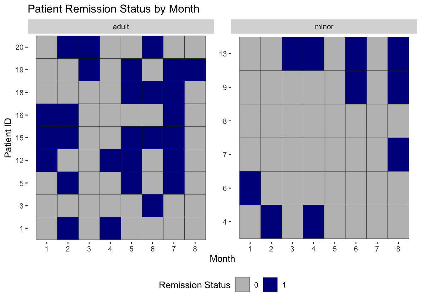

Forest Plots

# visualize exploratory variable Odds Radios from logistic regressions with biometrics dataset

# put ORs and CIs into dataframes, create outcome variable
OR_thigh_overweight <- tidy(thigh_overweight, exponentiate = TRUE, conf.int = TRUE) %>%
  mutate(outcome = "overweight")
OR_thigh_obese <- tidy(thigh_obese, exponentiate = TRUE, conf.int = TRUE) %>%
  mutate(outcome = "obese")
OR_wrist_overweight <- tidy(wrist_overweight, exponentiate = TRUE, conf.int = TRUE) %>%
  mutate(outcome = "overweight")
OR_wrist_obese <- tidy(wrist_obese, exponentiate = TRUE, conf.int = TRUE) %>%
  mutate(outcome = "obese")
OR_waist_overweight <- tidy(waist_overweight, exponentiate = TRUE, conf.int = TRUE) %>%
  mutate(outcome = "overweight")
OR_waist_obese <- tidy(waist_obese, exponentiate = TRUE, conf.int = TRUE) %>%
  mutate(outcome = "obese")

# combine OR dataframes to plot
all_ORs <- OR_thigh_overweight %>%
  bind_rows(OR_thigh_obese) %>%
  bind_rows(OR_wrist_overweight) %>%
  bind_rows(OR_wrist_obese) %>%
  bind_rows(OR_waist_overweight) %>%
  bind_rows(OR_waist_obese) %>%
# filter to only predictors of interest
  filter(str_detect(term, "girth")) %>%
# labels for plot
  mutate(term_lab = str_remove(term, "_girth")) %>%
  mutate(outcome_lab = if_else(outcome == "obese", 
                               "Obese (BMI>=30)", "Overweight (BMI>=25)"))

# create forest plot summary of ORs
ggplot(data = all_ORs) +
  geom_point(aes(x = estimate, y = term_lab)) +
  geom_errorbar(aes(xmin = conf.low, xmax = conf.high, y = term_lab), width = 0.2) +
        # width to change width of error bars
  facet_wrap(~outcome_lab, ncol = 1) +
  labs(x = "Odds Ratio", y = "Girth (cm)") + 
  geom_vline(aes(xintercept = 1.0), linetype = "dashed") +
  scale_x_continuous(breaks = seq(from=0.0, to=5.0, by=0.5), limits = c(0,5)) +
  theme_bw()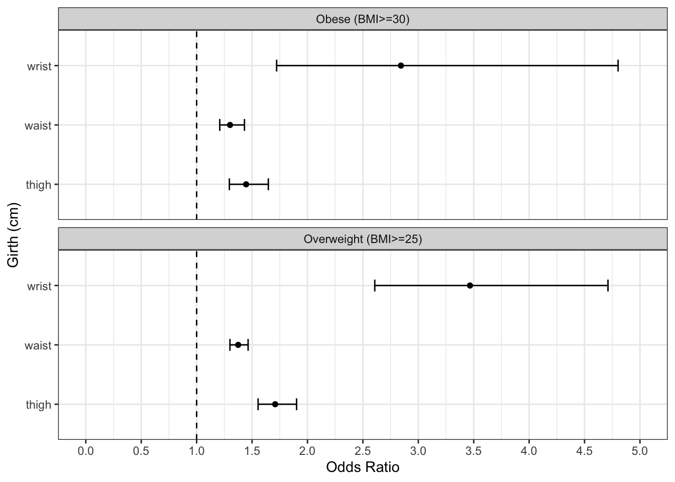

Custom/Mixed Plots

# shows the proportion of compliant individuals and 95% confidence interval per week over target compliance rate from compliance dataset
ggplot(data = proportion_by_week) +
  geom_pointrange(aes(x = week, y = compliance_proportion, ymax = upper_ci, ymin = lower_ci)) + 
  geom_line(aes(x = week, y = compliance_proportion), linetype = "dotted") +
  geom_hline(aes(yintercept = 0.65), color = "darkblue", linetype = "dashed") +
  theme_bw() +
  labs(title = "Observed Proportion of Compliant Individuals by Week", 
       x = "Week", y = "Proportion") +
  scale_x_continuous(breaks = 1:10, labels = paste("Week", 1:10)) +
  scale_y_continuous(limits = 0:1) +
  annotate(geom = "text", x = 8, y = 0.9, label = "Target Compliance = 0.65", 
           color = "darkblue")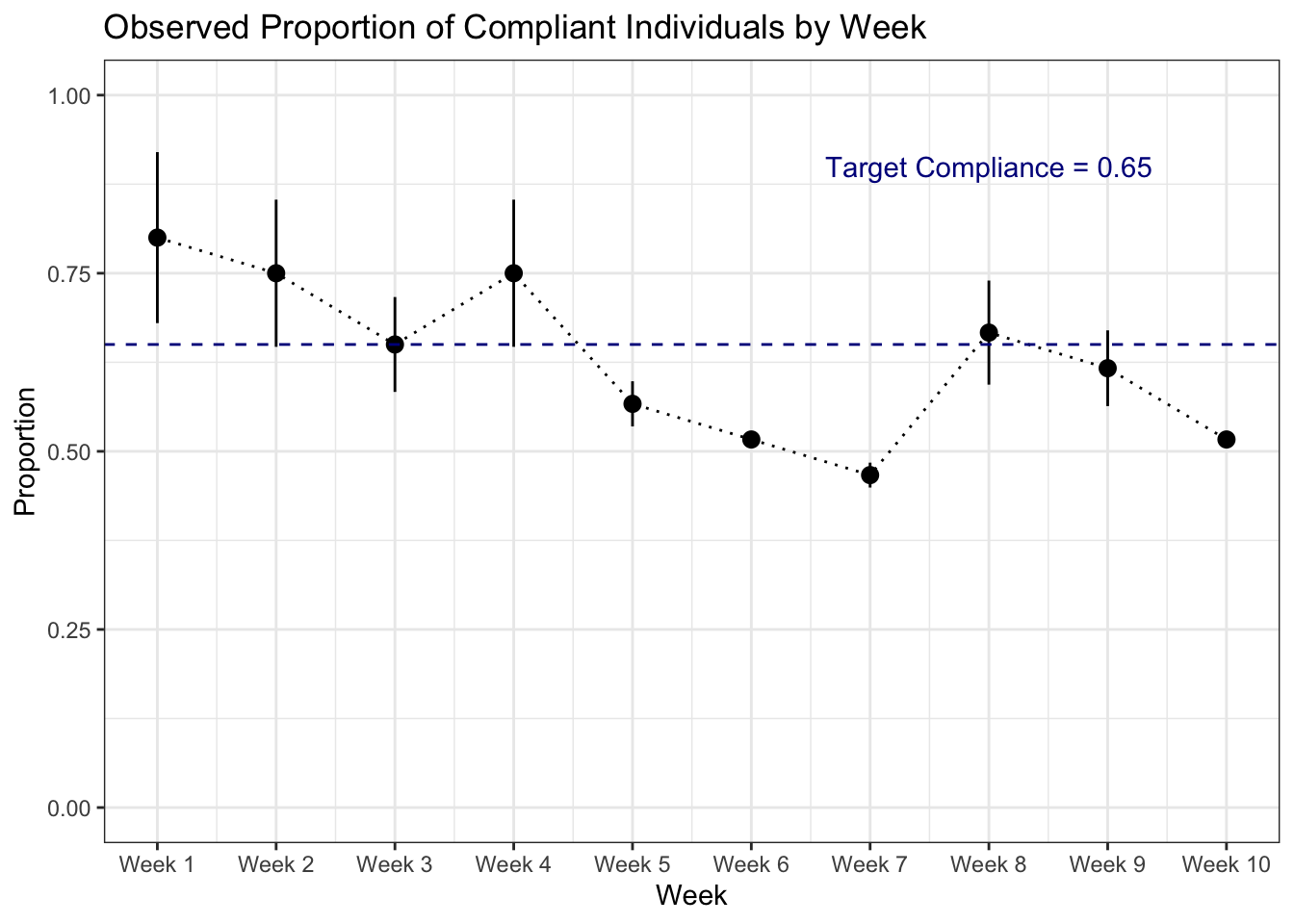

# patchwork plot showing patient trajectories over time, faceted by minor status from OCD dataset
lasagna <- ggplot(data = ocd_long) +
  geom_tile(aes(x = month, y = study_id, fill = rem_fac), color = "black") +
  labs(x = "Month", y = "Patient ID", title = "Patient Remission Status by Month",
       fill = "Remission Status") +
  theme(legend.position = "bottom",
        panel.background = element_rect(fill="white")) +
  scale_x_continuous(breaks = 1:8) +
  scale_fill_manual(values = c("grey", "darkblue")) +
  facet_wrap(~age_cat, scales = "free")

spaghetti <- ggplot(data = ocd_long) +
  geom_line(aes(x = month, y = ybocs_score, group = study_id), alpha=0.5) + 
  theme_bw() +
  labs(x = "Month", y = "YBOCS Score", title = "Patient YBOCS Scores by Month") +
  scale_x_continuous(breaks = 1:8, labels = scales::label_number(prefix = "Month ")) +
  facet_wrap(~age_cat)

lasagna / spaghetti +
  plot_annotation(title = "Patient Trajectories",
                  theme = theme(plot.title = element_text(size=rel(1.5), face="bold")))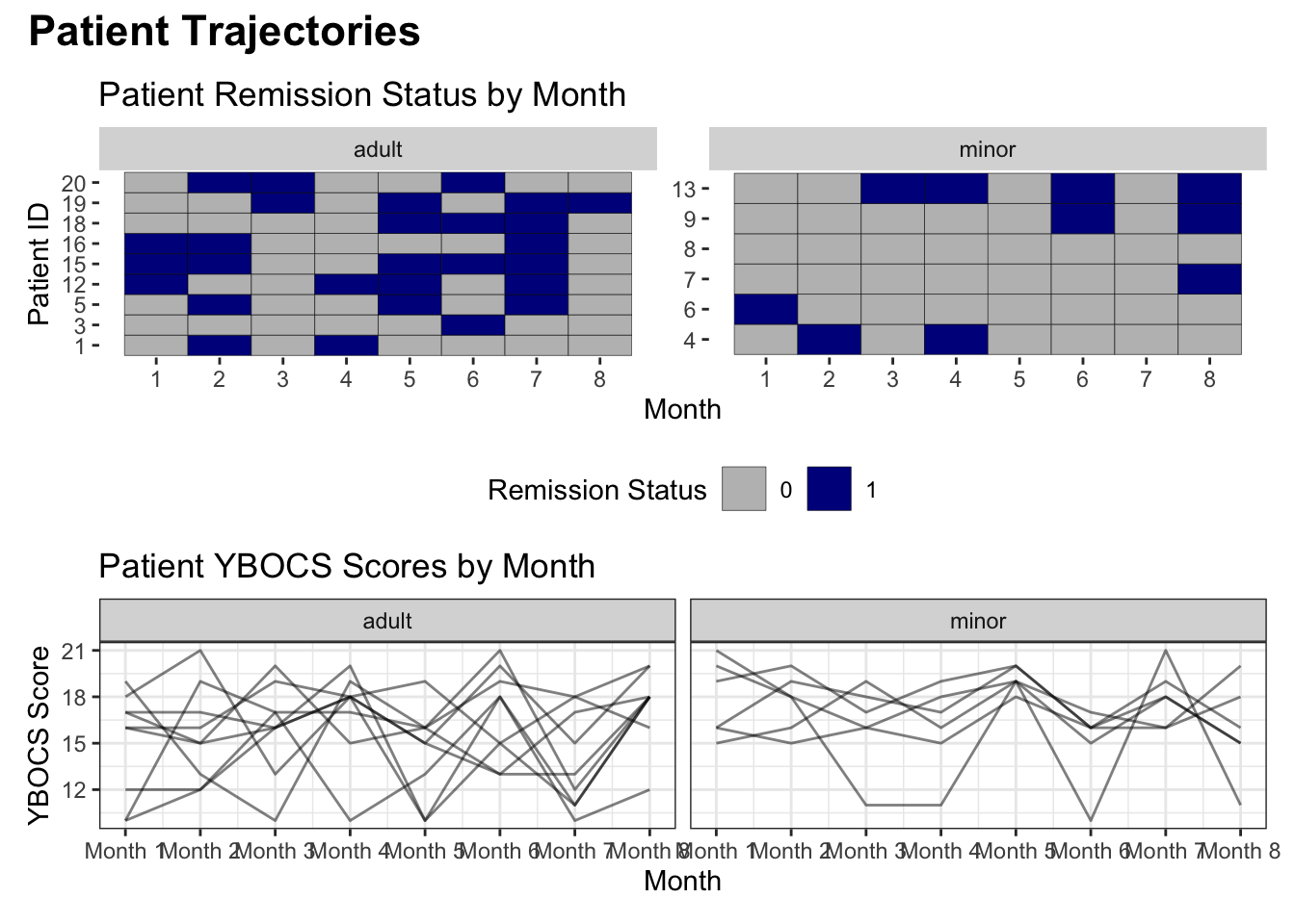

Descriptive Tables

# labeled table presenting mean, standard deviation, minimum, median, maximum, p-value of t-test of continuous variables, split by gender
biometrics_raw %>%
  select(gender, contains("girth")) %>%
  tbl_summary(by = gender,
    statistic = all_continuous() ~ "{mean} ({sd}), {min} {median} {max}",
                  label = list(shoulder_girth ~ "Shoulder Girth",
                           chest_girth ~ "Chest Girth",
                           waist_girth ~ "Waist Girth",
                           navel_girth ~ "Navel Girth",
                           hip_girth ~ "Hip Girth",
                           thigh_girth ~ "Thigh Girth",
                           bicep_girth_flexed ~ "Flexed Bicep Girth",
                           forearm_girth ~ "Forearm Girth",
                           knee_girth ~ "Knee Girth",
                           calf_girth ~ "Calf Girth",
                           ankle_girth ~ "Ankle Girth",
                           wrist_girth ~ "Wrist Girth")) %>% 
  add_p(test = all_continuous() ~ "t.test",
        test.args = all_tests("t.test") ~ list(var.equal = TRUE))

Characteristic	Female, N = 260¹	Male, N = 247¹	p-value²
Shoulder Girth	100 (6), 86 100 130	117 (6), 100 116 135	<0.001
Chest Girth	86 (6), 73 86 109	101 (7), 79 101 119	<0.001
Waist Girth	70 (8), 58 68 102	85 (9), 67 83 113	<0.001
Navel Girth	84 (10), 64 82 121	88 (8), 67 87 112	<0.001
Hip Girth	96 (7), 79 95 128	98 (6), 82 97 119	<0.001
Thigh Girth	57.2 (4.6), 46.3 56.4 75.7	56.5 (4.2), 46.8 56.0 70.0	0.078
Flexed Bicep Girth	28.1 (2.7), 22.4 27.8 40.3	34.4 (3.0), 25.6 34.4 42.4	<0.001
Forearm Girth	23.76 (1.68), 19.60 23.60 30.80	28.24 (1.78), 22.70 28.40 32.50	<0.001
Knee Girth	35.26 (2.58), 29.00 35.00 49.00	37.20 (2.27), 31.10 37.00 45.70	<0.001
Calf Girth	35.01 (2.61), 28.40 34.85 45.40	37.21 (2.65), 28.90 37.30 47.70	<0.001
Ankle Girth	21.21 (1.44), 17.40 21.10 26.00	23.16 (1.73), 16.40 23.00 29.30	<0.001
Wrist Girth	15.06 (0.85), 13.00 15.00 18.20	17.19 (0.91), 14.60 17.10 19.60	<0.001
¹ Mean (SD), Minimum Median Maximum
² Two Sample t-test

Machine Learning

Bootstrapping

# Obtain 95% confidence interval around a mean using standard SE formula

# Get mean of new COVID-19 deaths in NYC in 2022
ny_covid22 <- covid_raw %>%
# filter to NY
  filter(state == "New York") %>%
  arrange(date) %>%
# calculate new deaths
  mutate(new_deaths = deaths - lag(deaths)) %>%
# filter to dates in year 2022
  filter(date >= "2022-01-01")

mean_nd <- ny_covid22 %>%
  pull(new_deaths) %>%
  mean()

standard_ci <- ny_covid22 %>%
  summarize(mean_nd = mean(new_deaths),
            total_n = n(),
            se = sd(new_deaths)/sqrt(total_n),
            lower_ci = mean_nd - 1.96*se,
            upper_ci = mean_nd + 1.96*se) %>%
  mutate(pretty_ci = str_c(round(mean_nd,2), " (", round(lower_ci,2), ", ", round(upper_ci,2), ")"))

ci_out <- standard_ci %>%
  pull(pretty_ci)

The mean number and 95% confidence interval of daily new COVID-19 deaths reported in New York since 01/01/2022 is 47.24 (30, 64.47).

# Obtain 95% confidence interval around a mean using bootstrapping

# create functions
get_mean <- function(df){
  mean <- df %>%
    pull(new_deaths) %>%
    mean()
  return(mean)
}
create_bootstrap <- function(df){
  boot <- df %>%
    slice_sample(prop = 1, replace = TRUE) # pull sample the same size as original
  return(boot)
}
# combine functions
mean_bootstrap <- function(df){
  boot_m <- create_bootstrap(df) %>%
    get_mean()
  return(boot_m)
}

# get boostrapped results and put into a tibble
boot_res <- map_dbl(1:2000, function(x) mean_bootstrap(ny_covid22))
res_tibble <- tibble(run = 1:2000, mean = boot_res)

# get boostrapped confidence interval with quantiles
boot_ci <- res_tibble %>%
  summarize(lower_ci = quantile(mean, 0.025),
         upper_ci = quantile(mean, 0.975))

# plot the distribution of boostrapped data
ggplot(data = res_tibble) +
  geom_histogram(aes(x = mean), color = "white", fill = "darkgrey") +
  theme_bw() +
  labs(title = "Bootstrapped Distribution")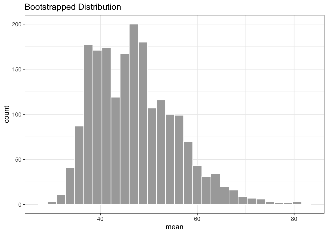

The bootstrapped 95% CI for number of new deaths reported in New York from 01/01/22 onward is 34.533557, 66.3423937.

Predictive Model Building

Using k-fold cross validation, CART modeling, and logistic regression modeling

# Step 1: Split data into training and test sets

biometrics_pred <- biometrics_log %>%
# factor outcome and gender
  mutate(gender_fac = factor(gender, levels = c('Female', 'Male')),
         wt = if_else(overweight == 0, 'Not_overweight', 'Overweight'),
         wt_fac = factor(wt, levels = c('Not_overweight', 'Overweight'))) %>%
# remove variables
  select(-id, -obese, -overweight, -age, -weight, -wt, -height, -bmi, -gender)

# check distribution of outcome overweight in total dataset
biometrics_pred %>%
  group_by(wt_fac) %>%
  summarize(n = n()) %>%
  mutate(proportion = n / sum(n))

## # A tibble: 2 × 3
##   wt_fac             n proportion
##   <fct>          <int>      <dbl>
## 1 Not_overweight   357      0.704
## 2 Overweight       150      0.296

#split data, 75% training
split_data <- initial_split(biometrics_pred, prop = 0.75, strata = wt_fac)
      # stratify so proportion of outcome is the same between training/test
train_dat <- training(split_data)
test_dat <- testing(split_data)

# Check that distribution of outcome is similar to total dataset in training and test sets
train_dat %>%
  group_by(wt_fac) %>%
  summarize(n = n()) %>%
  mutate(proportion = n / sum(n))

## # A tibble: 2 × 3
##   wt_fac             n proportion
##   <fct>          <int>      <dbl>
## 1 Not_overweight   267      0.704
## 2 Overweight       112      0.296

test_dat %>%
  group_by(wt_fac) %>%
  summarize(n = n()) %>%
  mutate(proportion = n / sum(n))

## # A tibble: 2 × 3
##   wt_fac             n proportion
##   <fct>          <int>      <dbl>
## 1 Not_overweight    90      0.703
## 2 Overweight        38      0.297

The distribution of outcome (overweight) in the training and test data appears equal.

logistic_mod <- train(
  form = wt_fac ~ ., # formula
  data = train_dat,  # training data
  trControl = trainControl(method = "cv", # cross-validation
                           number = 10, # 10-fold 
                           summaryFunction = twoClassSummary, # obtain ROC
                           classProbs = TRUE, # obtain ROC
                           savePredictions = "final"), # plot ROC/AUC
  metric = "ROC", # use ROC/AUC
  method = "glm", # glm function
  family = "binomial" # logistic regression
)

The 10-fold cross-validated ROC/AUC (10-fold) of this model on the training dataset is 0.968839.

## tune based on ROC/AUC
class_tree <- train(
  form = wt_fac ~ ., # formula
  data = train_dat, # training data
  method = "rpart", # CART
  trControl = trainControl(method = "cv", # cross validation
                           number = 10, # 10-fold
                           summaryFunction = twoClassSummary, # obtain ROC
                           classProbs = TRUE, # obtain ROC
                           savePredictions = "final"), # save for plotting ROC/AUC
  metric = "ROC" # use ROC/AUC
  )

# cross-validated model ROC/AUC vs different complexity parameters
plot(class_tree)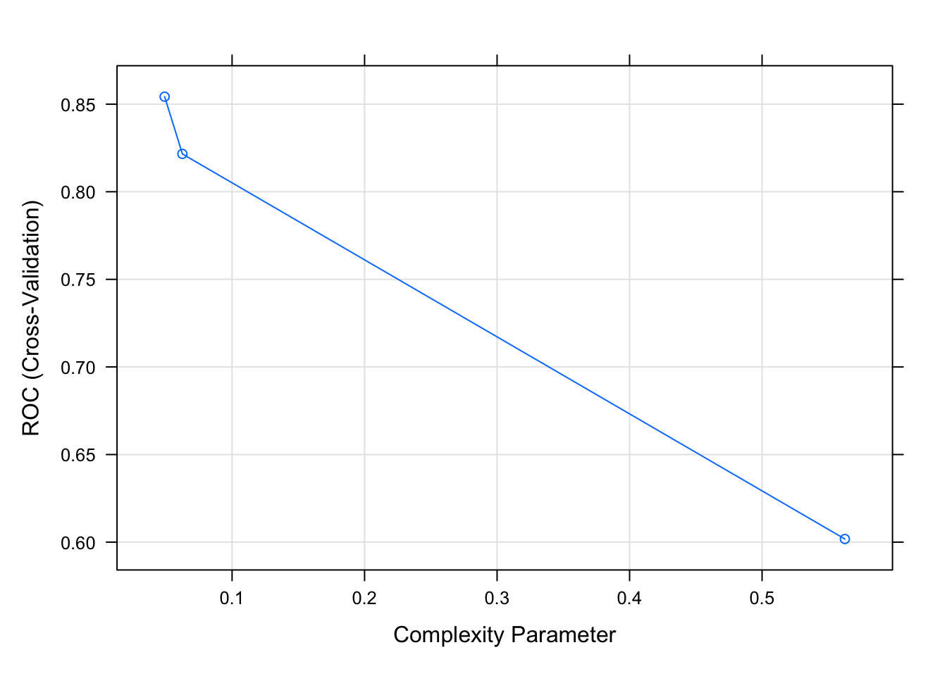

The best reported ROC/AUC value to maximize performance is 0.0491071.

# plot final model
rpart.plot(class_tree$finalModel)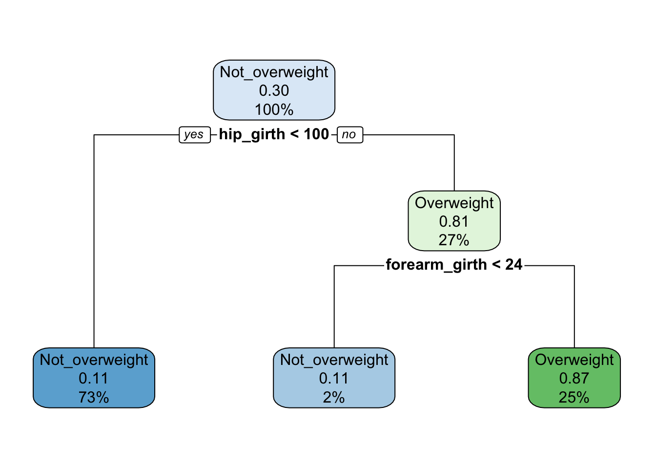


# compare cross-validated ROC/AUC of logistic and CART to see which model is best
compare_mods <- resamples(list("Logistic"=logistic_mod, 
                             "CART" = class_tree))

dotplot(compare_mods, metric = "ROC")

The logistic model performs better on the training data with the AUC=0.97 compared to 0.85.

# create a ROC plot and report the AUC for final logistic model on the test set
log_pred_prob <- predict(logistic_mod, newdata = test_dat, type = "prob") 
        # type = "prob" gives predicted probabilities

# merge datasets
log_test_pred_df <- test_dat %>%
  bind_cols(log_pred_prob)

log_test_roc <- roc(wt_fac ~ Overweight, data = log_test_pred_df)

# plot ROC values
ggroc(log_test_roc) +
  theme_bw()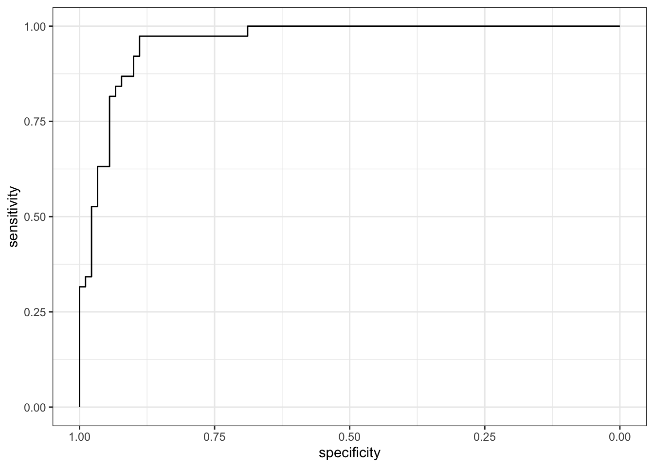

The AUC for my final logistic model is 0.9588.

This is a high AUC value and suggests the model performs strongly on the test data.

R Code Samples